sRGB#

colorsynth.sRGB(XYZ, axis=-1)[source]#

Convert CIE 1931 tristimulus values, calculated using XYZcie1931_from_spd(), into the sRGB color space, the standard color space used on computer monitors.

Parameters:

XYZ (ndarray) – the CIE 1931 tristimulus values, \(XYZ\).
axis (int) – the axis along which the different tristimulus values are arranged

Return type:

ndarray

Examples

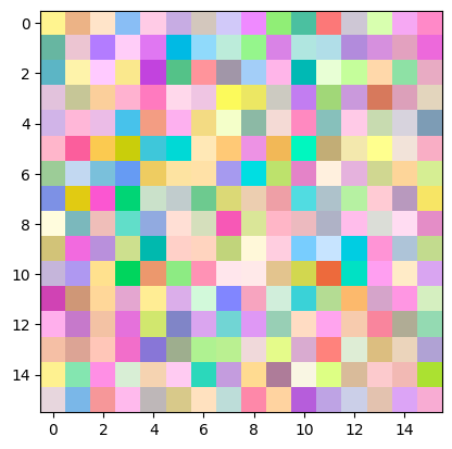
Plot a 2d set of random spectral power distribution curves as a color image

import numpy as np
import matplotlib.pyplot as plt
import astropy.units as u
import colorsynth

# Define the number of wavelength bins in our spectrum
num = 11

# Define an evenly-spaced grid of wavelengths
wavelength = np.linspace(380, 780, num=num) * u.nm

# Define a random spectral power distribution cube by sampling from a uniform distribution
spd = np.random.uniform(size=(16, 16, num))

# Calculate the CIE 1931 tristimulus values from the spectral power distribution
XYZ = colorsynth.XYZcie1931_from_spd(spd, wavelength)

# Normalize the tristimulus values based on the max value of the Y parameter
XYZ = XYZ / XYZ[..., 1].max()

# Convert the tristimulus values into sRGB, the standard used in most
# computer monitors
rgb = colorsynth.sRGB(XYZ)

# Plot the result as an image
plt.figure();
plt.imshow(rgb);

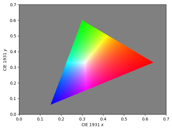
Plot the sRGB color gamut, the complete subset of colors that can be reproduced accurately with sRGB.

# Define a grid of CIE xy values
x = np.linspace(0, 0.7, num=1000)[:, np.newaxis]
y = np.linspace(0, 0.7, num=1001)[np.newaxis, :]

# Define a very small value for the luminance,
# so that the gamut is as large as possible
Y = 1e-3

# Define an axis which represents the
# components of the color vectors
axis = -1

# Create a CIE 1931 xyY color vector
xyY = np.stack(np.broadcast_arrays(x, y, Y), axis=axis)

# Convert the color space from CIE 1931 xyY to XYZ
XYZ = colorsynth.XYZ_from_xyY_cie(xyY, axis=axis)

# Convert the color space again from CIE 1931 XYZ
# to our target, sRGB.
rgb = colorsynth.sRGB(XYZ, axis=axis)

# Find the pixels that are within the sRGB gamut
# by checking if they are finite, and if they lie within the range 0-1.
where_nan = ~np.all(np.isfinite(rgb), axis=axis, keepdims=True)
where_invalid = ~np.all((0 <= rgb) & (rgb <= 1), axis=axis, keepdims=True)
where_outside = where_nan | where_invalid
where_outside = np.broadcast_to(where_outside, rgb.shape)
where_inside = ~where_outside

# Set the pixels outside the gamut to gray
rgb[where_outside] = 0.5

# Scale the RGB values inside the gamut to the most saturated
# color possible
rgb[where_inside] = (rgb / np.max(rgb, axis=axis, keepdims=True))[where_inside]

# plot the sRGB gamut
plt.figure();
plt.pcolormesh(
    *np.broadcast_arrays(x, y),
    np.moveaxis(rgb, source=axis, destination=-1),
);
plt.xlabel("CIE 1931 $x$");
plt.ylabel("CIE 1931 $y$");

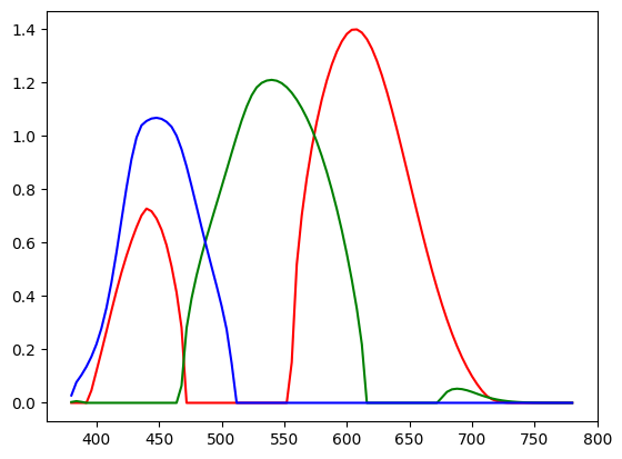
Plot the response curves of the \(R\), \(G\), and \(B\) to a constant spectral power distribution

# Define an evenly-spaced grid of wavelengths
wavelength = np.linspace(380, 780, num=101) * u.nm

spd = np.diagflat(np.ones(wavelength.shape))

# Calculate the CIE 1931 tristimulus values from the spectral power distribution
XYZ = colorsynth.XYZcie1931_from_spd(spd, wavelength[..., np.newaxis], axis=0)

# Normalize the tristimulus values based on the max value of the Y parameter
XYZ = XYZ / XYZ.max(axis=1, keepdims=True)
XYZ = XYZ * np.array([0.9505, 1.0000, 1.0890])[..., np.newaxis]

# Convert the tristimulus values into sRGB
r, g, b = np.clip(colorsynth.sRGB(XYZ, axis=0), 0, 10)

plt.figure();
plt.plot(wavelength, r, color="red");
plt.plot(wavelength, g, color="green");
plt.plot(wavelength, b, color="blue");

sRGB#

This Page