Introduction#

colorsynth is a Python library for creating false-color images from spectral cubes: arrays with two spatial axes and one spectral axis, such as those measured by scanning-slit spectrographs. It collapses the spectral axis of a numpy.ndarray into red, green, and blue (\(RGB\)) channels that can be displayed on your computer monitor by mapping the spectrum into the human visible range and weighting it by the CIE 1931 color-matching functions. The shape of the spectrum controls the hue of each pixel, and the total intensity controls its brightness, so features like Doppler shifts are visible directly in the image.

Installation#

colorsynth is available on the PyPI and can be installed using pip:

pip install colorsynth

A simple example#

The main entry point of this library is colorsynth.rgb(), which converts a spectral cube into an RGB image.

The cube below contains a Gaussian emission line at every point, with a center wavelength that increases from left to right, and a total intensity that increases from top to bottom. In the resulting false-color image, the center wavelength of the line appears as hue, and its total intensity appears as brightness.

import numpy as np
import matplotlib.pyplot as plt
import astropy.units as u
import colorsynth

# Define a wavelength grid for the spectral axis
wavelength = np.linspace(400, 700, num=61) * u.nm

# Define a spatial grid
x = np.linspace(0, 1, num=101)[:, np.newaxis, np.newaxis]
y = np.linspace(0, 1, num=101)[np.newaxis, :, np.newaxis]

# Define a spectral cube containing a Gaussian emission line
# at every point, with a center wavelength that increases from
# left to right, and a total intensity that increases from top
# to bottom
center = 420 * u.nm + (680 - 420) * u.nm * y
width = 15 * u.nm
spd = x * np.exp(-np.square((wavelength - center) / width))

# Collapse the wavelength axis of the cube into RGB channels
rgb = colorsynth.rgb(spd, wavelength, axis=~0, spd_min=0, spd_max=1)

# Display the result as a false-color image
fig, ax = plt.subplots(constrained_layout=True)
ax.imshow(rgb);

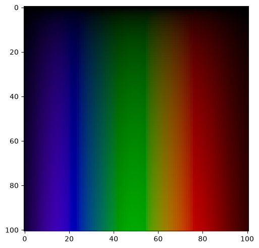
The spd_min and spd_max arguments fix the range of the intensity normalization for the whole cube. If they are omitted, every wavelength bin is normalized independently by its own minimum and maximum over the spatial axes, which is often useful for real data with a bright continuum, but would exaggerate the faint wings of the emission line in this synthetic example.

Gallery#

The examples below show how the shape of a spectral power distribution (SPD) determines the color computed by colorsynth.rgb(). In each panel, the area under the SPD is filled with the color that colorsynth computes for that spectrum.

Narrow emission lines produce the saturated spectral hues, a doublet mixes the hues of its components (blue plus red makes purple, a color that no single wavelength can produce), and broadband spectra wash out toward white: the flat spectrum is nearly neutral, while the blackbody curves are warm or cool tints depending on whether the red or blue end dominates.

import numpy as np
import matplotlib.pyplot as plt
import astropy.units as u
import astropy.constants
import astropy.visualization
import colorsynth

# Define a wavelength grid spanning the human visible range
wavelength = np.linspace(380, 700, num=321) * u.nm

def gaussian(center: u.Quantity, width: u.Quantity) -> np.ndarray:
    """A Gaussian emission line with the given center and width."""
    return np.exp(-np.square((wavelength - center) / width))

def blackbody(temperature: u.Quantity) -> np.ndarray:
    """A normalized Planck spectrum for the given temperature."""
    h = astropy.constants.h
    c = astropy.constants.c
    k_B = astropy.constants.k_B
    spd = 1 / wavelength**5 / np.expm1(h * c / (wavelength * k_B * temperature))
    return (spd / spd.max()).to_value(u.dimensionless_unscaled)

# A collection of example spectral power distributions
spds = {
    "blue emission line": gaussian(450 * u.nm, 10 * u.nm),
    "green emission line": gaussian(540 * u.nm, 10 * u.nm),
    "red emission line": gaussian(620 * u.nm, 10 * u.nm),
    "blue + red doublet": gaussian(450 * u.nm, 10 * u.nm) + gaussian(640 * u.nm, 10 * u.nm),
    "broad emission line": gaussian(550 * u.nm, 80 * u.nm),
    "flat spectrum": np.ones(wavelength.shape),
    "3000 K blackbody": blackbody(3000 * u.K),
    "20000 K blackbody": blackbody(20000 * u.K),
}

# Plot each spectral power distribution, filling the area under
# the curve with the color computed by colorsynth
with astropy.visualization.quantity_support():
    fig, axs = plt.subplots(
        nrows=4,
        ncols=2,
        figsize=(8, 8),
        sharex=True,
        constrained_layout=True,
    )
    for ax, (label, spd) in zip(axs.flat, spds.items()):
        color = colorsynth.rgb(
            spd,
            wavelength,
            axis=-1,
            spd_min=0,
            spd_max=spd.max(),
        )
        ax.set_facecolor("0.85")
        ax.fill_between(wavelength, spd, color=color)
        ax.plot(wavelength, spd, color="black", linewidth=0.5)
        ax.set_title(label, fontsize=10)
        ax.set_ylim(0, 1.1)
    for ax in axs[~0]:
        ax.set_xlabel(f"wavelength ({wavelength.unit:latex_inline})")
    for ax in axs[:, 0]:
        ax.set_ylabel("relative intensity")

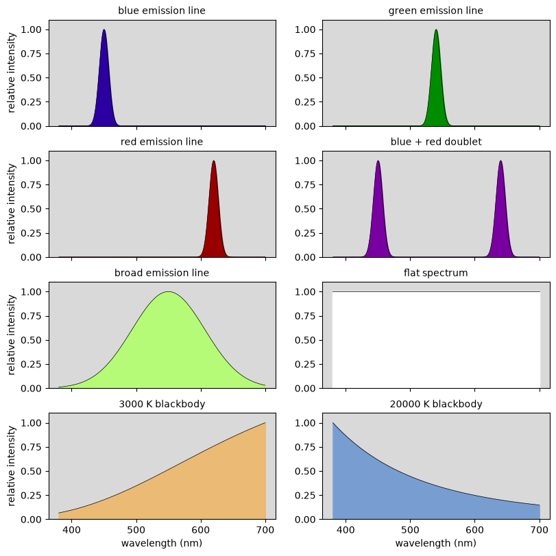
Note that the saturated colors of the narrow emission lines are limited by the sRGB gamut of a computer monitor: a truly monochromatic green, for example, lies outside the gamut, so colorsynth.rgb() clips it to the closest displayable color.

Colorizing IRIS spectroheliograms#

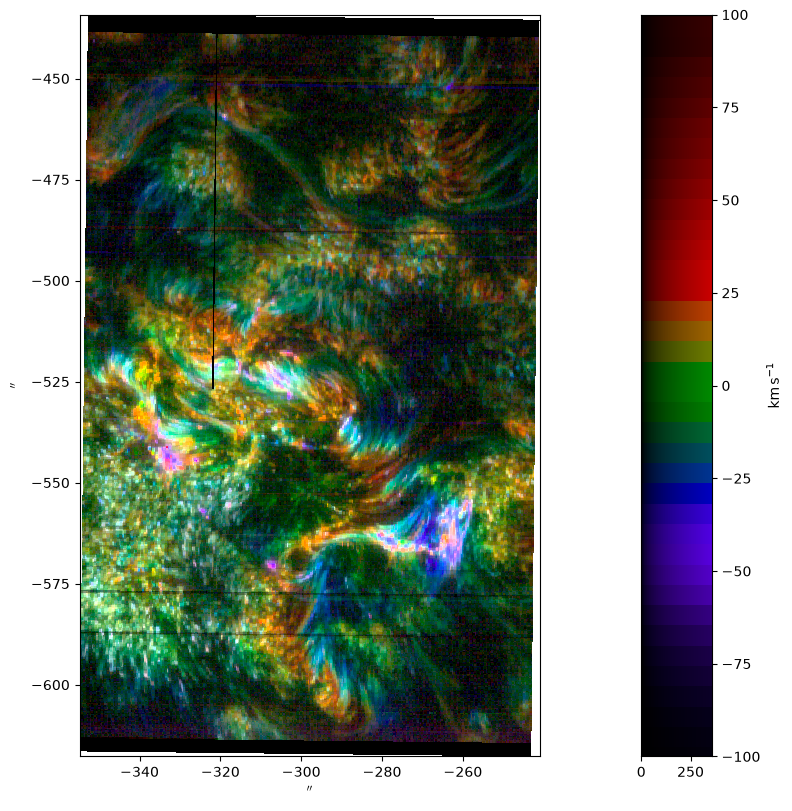
The Interface Region Imaging Spectrograph (IRIS), is a NASA Small Explorer satellite that has been observing the Sun in ultraviolet since 2013.

IRIS is a scanning slit spectrograph which allows it to capture a 3D data product in \(x\), \(y\) and wavelength. Visualizing this 3D data on a 2D computer monitor presents obvious difficulties. With colorsynth, we can plot this type of data using color as a third dimension.

import shutil
import urllib
import pathlib
import numpy as np
import matplotlib.pyplot as plt
import scipy.ndimage
import astropy.units as u
import astropy.visualization
import astropy.wcs
import astropy.io
import astroscrappy
import colorsynth

# Download tar.gz archive containing IRIS raster FITS files
archive, _ = path, headers = urllib.request.urlretrieve(
    url=r"https://www.lmsal.com/solarsoft/irisa/data/level2_compressed/2021/09/23/20210923_061339_3620108077/iris_l2_20210923_061339_3620108077_raster.tar.gz",
    filename="raster.tar.gz",
)

# Unpack tar.gz archive into folder
directory = pathlib.Path("raster")
shutil.unpack_archive(filename=archive, extract_dir=directory)
fits = list(directory.glob("*.fits"))

# Open FITS file containing IRIS spectroheliograms
hdu_list = astropy.io.fits.open(fits[0])
hdu = hdu_list[4]

# Create World Coordinate System instance from the FITS header
wcs = astropy.wcs.WCS(hdu)

# Determine the physical meaning of each axis in the FITS file
axes = list(reversed(wcs.axis_type_names))
axis_x = axes.index("HPLN")
axis_y = axes.index("HPLT")
axis_wavelength =  axes.index("WAVE")
axis_xy = (axis_x, axis_y)

# Save spectroheliogram data to a local variable
spd = hdu.data
where_valid = spd > -10
spd[~where_valid] = 0

# Remove cosmic ray spikes from the spectroheliogram
for i in range(spd.shape[0]):
    spd[i] = astroscrappy.detect_cosmics(spd[i], cleantype="medmask")[1]

# Calculate an estimate of the stray light in the spectroheliogram
bg = np.median(spd, axis=0)
bg = scipy.ndimage.median_filter(bg, size=(31, 151))
bg = scipy.ndimage.uniform_filter(bg, size=31)

# Remove the stray light from the spectroheliogram
spd = spd - bg
spd[~where_valid] = 0

# Calculate coordinate arrays in wavelength and helioprojective x/y
wavelength, hy, hx = wcs.array_index_to_world(*np.indices(spd.shape))
hx = hx << u.arcsec
hy = hy << u.arcsec
wavelength = wavelength << u.AA

# Convert wavelength coordinates to Doppler shift
wavelength_center = hdu_list[0].header["TWAVE4"] * u.AA
velocity = (wavelength - wavelength_center) * astropy.constants.c / wavelength_center
velocity = velocity.to(u.km / u.s)

# Define the velocity range to colorize
velocity_min = -100 * u.km / u.s
velocity_max = +100 * u.km / u.s

# Convert spectroheliogram to an RGB image
rgb, colorbar = colorsynth.rgb_and_colorbar(
    spd=spd,
    wavelength=velocity.mean(axis_xy, keepdims=True),
    axis=axis_wavelength,
    spd_min=0,
    spd_max=np.percentile(spd, 99, axis=axis_xy, keepdims=True),
    wavelength_min=velocity_min,
    wavelength_max=velocity_max,
    wavelength_norm=lambda x: np.arcsinh(x / (25 * u.km / u.s))
)

# Plot the RGB image
with astropy.visualization.quantity_support():
    fig, axs = plt.subplots(
        ncols=2,
        figsize=(8, 8),
        gridspec_kw=dict(width_ratios=[.9,.1]),
        constrained_layout=True,
    )
    axs[0].pcolormesh(
        hx.mean(axis_wavelength),
        hy.mean(axis_wavelength),
        np.clip(np.moveaxis(rgb, axis_wavelength, ~0), 0, 1),
    )
    axs[0].set_aspect("equal")
    axs[1].pcolormesh(*colorbar)
    axs[1].yaxis.tick_right()
    axs[1].yaxis.set_label_position("right")
    axs[1].set_ylim(velocity_min, velocity_max)

Citation#

If you use colorsynth in your research, please cite it. The citation metadata is kept in CITATION.cff, which the “Cite this repository” button on the GitHub page can export as BibTeX or APA. Please include the version of colorsynth that you used, which is given by importlib.metadata.version("colorsynth").

@software{colorsynth,
  author = {Smart, Roy T.},
  title = {colorsynth},
  version = {X.Y.Z},
  url = {https://github.com/sun-data/colorsynth},
}

API Reference#

colorsynth

Create false-color images from spectral cubes.

Bibliography#

[1]

CIE. Colorimetry. Commission Internationale de l'Éclairage, Vienna, Austria, 3 edition, 2004. ISBN 978-3-901906-33-6. CIE 15:2004.